Topic
Descriptive Statistics: Definition, Types and Examples
What descriptive statistics are, the four types and their measures, one dataset described from start to finish, and how to choose what to report.
By Hira Noor, BS Mathematics · Updated · 10 min read
Definition
Descriptive statistics are numbers, tables and graphs that summarize the data you actually have, without generalizing beyond it. They fall into four types: frequency (counts and percentages), central tendency (mean, median, mode), variability (range, variance, standard deviation, IQR) and position (percentiles, quartiles, z-scores). Inferential statistics, by contrast, use a sample to draw conclusions about a larger population.
Key takeaways
- Descriptive statistics describe a dataset; they do not test hypotheses or generalize to a population.
- The four types are frequency, central tendency, variability and position. Shape (skewness and kurtosis) is often added as a fifth.
- A useful summary always pairs a measure of center with a measure of spread: mean with standard deviation, or median with IQR.
- Use the mean and standard deviation for symmetric data, and the median and IQR for skewed data or data with outliers.
- Tables (frequency tables) and graphs (histograms, box plots, bar charts) are descriptive statistics too.
- ANOVA, t-tests, p-values and confidence intervals are inferential, not descriptive.
On this page
- What is descriptive statistics?
- The four types of descriptive statistics
- Worked example: describing one dataset
- Tables and graphs in descriptive statistics
- Univariate vs bivariate descriptive statistics
- Which descriptive statistics should you report?
- Descriptive vs inferential statistics
- Common mistakes with descriptive statistics
- Descriptive statistics guides
- FAQ
What is descriptive statistics?
Descriptive statistics is the branch of statistics that organizes and summarizes data so you can see what it looks like. A single descriptive statistic, such as an average, a percentage or a range, condenses many values into one number. A set of them, reported together with a table or a graph, gives a compact picture of a whole dataset: where its values cluster, how far they spread and whether any are unusual.
The key word is describe. Descriptive statistics report what is true of the values in front of you, and nothing more. When you use those values to estimate something about a larger group, such as every customer rather than the 200 you surveyed, you have moved into inferential statistics, which adds probability and uncertainty. The full comparison is in Descriptive vs Inferential Statistics: Differences and Examples.
Descriptive statistics are usually the first step of any analysis. Researchers report them in “Table 1” of a paper, businesses track them on dashboards, and teachers use them to summarize test results. To get every common summary for your own numbers in one table, paste them into the Descriptive Statistics Calculator.
Try it: Descriptive Statistics CalculatorPaste a dataset to get the mean, median, mode, SD, variance, quartiles, IQR, outliers, skewness and kurtosis in one table, with steps.The four types of descriptive statistics
Most textbooks group descriptive statistics into four types. Each one answers a different question about the same data, so a full summary normally uses at least one measure from each of the middle two.
| Type | Question it answers | Main measures |
|---|---|---|
| Frequency (distribution) | How often does each value or category occur? | Counts, percentages, relative and cumulative frequency |
| Central tendency | What is a typical value? | Mean, median, mode |
| Variability (dispersion) | How spread out are the values? | Range, interquartile range, variance, standard deviation, coefficient of variation |
| Position | Where does one value stand relative to the rest? | Percentiles, quartiles, z-scores, five-number summary |
1. Frequency distribution
A frequency distribution counts how many times each value, category or class interval appears. It is the only type that works for every kind of data, including categories such as blood type or product colour. Percentages (relative frequencies) make groups of different sizes comparable, and cumulative frequencies show how many values fall at or below a point. Build one from raw data with the Frequency Distribution Calculator.
2. Measures of central tendency
Central tendency describes the center of the data with one number. The mean adds the values and divides by how many there are, the median is the middle of the sorted values, and the mode is the most frequent value. The mean uses every value but is pulled by outliers; the median is not. Measures of Central Tendency: Mean, Median and Mode covers the formulas and when each one is the better choice.
3. Measures of variability
Variability (also called dispersion or spread) describes how far the values sit from each other and from the center. The range is the largest value minus the smallest. The interquartile range (IQR) is Q3 − Q1, the spread of the middle half. The variance is the average squared distance from the mean, and the standard deviation is its square root, in the original units. Two datasets can share a mean and still differ completely in spread, which is why a center on its own is never a full summary.
The n − 1 in the sample formula is Bessel’s correction; for a whole population you divide by N instead. Sample vs Population Standard Deviation: Which Should You Use? explains which one your data need. The Standard Deviation Calculator and Variance Calculator show both versions.
4. Measures of position
Measures of position locate a single value within the dataset. A percentile gives the percentage of values at or below it, quartiles split the sorted data into four equal parts (Q1, the median and Q3), and a z-score counts how many standard deviations a value lies from the mean. The five-number summary (minimum, Q1, median, Q3, maximum) combines position and spread and is what a box plot draws. Try the Percentile Calculator, Quartile Calculator or Z-Score Calculator.
Worked example: describing one dataset
The clearest way to see the four types working together is to apply them to one small dataset. Every value below can be checked in the Descriptive Statistics Calculator, whose default quartile method (median of the halves) matches the one used here.
Quiz scores for ten students
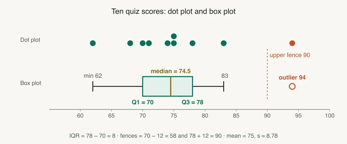
Problem. Ten students score 62, 68, 70, 71, 74, 75, 75, 78, 83 and 94 on a quiz (already sorted). Describe the scores.
- 01Frequency. n = 10. Every score appears once except 75, which appears twice.
- 02Mean. Σx = 750, so x̄ = 750 / 10 = 75.
- 03Median. n is even, so the median is the mean of the 5th and 6th values: (74 + 75) / 2 = 74.5.
- 04Mode. 75 is the only repeated score, so the mode is 75.
- 05Range. 94 − 62 = 32.
- 06Standard deviation. The deviations from 75 are −13, −7, −5, −4, −1, 0, 0, 3, 8, 19. Their squares sum to 694, so s² = 694 / (10 − 1) ≈ 77.11 and s = √77.11 ≈ 8.78.
- 07Quartiles and IQR. Lower half 62, 68, 70, 71, 74 gives Q1 = 70; upper half 75, 75, 78, 83, 94 gives Q3 = 78. IQR = 78 − 70 = 8.
- 08Outliers. The fences are Q1 − 1.5 × IQR = 58 and Q3 + 1.5 × IQR = 90. The score of 94 lies above 90, so it is an outlier.
Answer. Five-number summary: 62, 70, 74.5, 78, 94. The typical score is about 75 (mean 75, median 74.5), most scores sit within about 9 points of it (s ≈ 8.78), and one high score of 94 is an outlier that stretches the range and gives the data a slight right skew. For a report, the median and IQR (74.5 and 8) describe these scores more robustly than the mean and SD.
Tables and graphs in descriptive statistics
Descriptive statistics are not only numbers. A well-chosen table or graph shows the shape, gaps and outliers that a list of summary values can hide. The right display depends on whether your data are categories or numbers.
| Display | Data type | What it shows | Make one |
|---|---|---|---|
| Frequency table | Any | Counts and percentages for each value or class | Frequency table |
| Bar chart | Categorical | Counts or percentages compared across categories | Bar chart |
| Pie chart | Categorical | Each category’s share of a whole | Pie chart |
| Histogram | Numeric | Shape of the distribution: center, spread, skew, peaks | Histogram |
| Box plot | Numeric | Five-number summary and outliers; compares groups well | Box plot |
| Dot plot, stem-and-leaf plot | Numeric, small n | Every individual value with its frequency | Dot plot, stem-and-leaf |
| Scatter plot | Two numeric variables | Direction and strength of a relationship | Scatter plot |
Univariate vs bivariate descriptive statistics
Univariate descriptive statistics summarize one variable at a time: the mean height, the spread of exam scores, the share of each blood type. Bivariate descriptive statistics describe how two variables move together. For two numeric variables that means a scatter plot plus the correlation coefficient or covariance; for two categorical variables it means a cross-tabulation (contingency table) of counts. Describing more than two variables at once is multivariate description.
Which descriptive statistics should you report?
The level of measurement and the shape of the data decide which summaries are meaningful. Reporting a mean for categories, or a mean and SD for heavily skewed incomes, is a common mistake that this table helps avoid.
| Your data | Center | Spread | Good graph |
|---|---|---|---|
| Nominal (categories with no order) | Mode | Counts and percentages for each category | Bar chart |
| Ordinal (ordered categories, ratings) | Median (or mode) | Range or IQR | Bar chart |
| Numeric, roughly symmetric | Mean | Standard deviation | Histogram |
| Numeric, skewed or with outliers | Median | IQR (or the five-number summary) | Box plot or histogram |
Always report n alongside the summaries, and say which version of a formula you used where it matters (sample or population standard deviation, and the quartile method). Two people can compute different but equally valid Q1 and Q3 for the same data.
Descriptive vs inferential statistics
Descriptive statistics summarize the data you collected; inferential statistics use a sample to make claims about the population it came from. The same number can play either role: a sample mean of 75 is a descriptive statistic of your ten students, and it becomes inferential the moment you use it to estimate the mean of all students, with a confidence interval or a t-test. Population vs Sample: Definitions, Differences and Examples and Parameter vs Statistic: Difference, Symbols and Examples explain the vocabulary.
| Descriptive statistics | Inferential statistics | |
|---|---|---|
| Goal | Summarize the data you have | Generalize from a sample to a population |
| Typical output | Mean, SD, percentages, tables, graphs | Confidence intervals, p-values, test decisions |
| Uncertainty | None: the numbers are exact for this data | Quantified with probability |
| Examples | Mean, median, IQR, correlation, histogram | t-test, ANOVA, chi-square test, regression inference |
Common mistakes with descriptive statistics
- Reporting a center without a spread. A mean of 75 means little until you know whether scores ranged from 74 to 76 or from 20 to 100.
- Using the mean for skewed data. Incomes, house prices and waiting times are right-skewed, so the median is the more typical value.
- Mixing up n and n − 1. Spreadsheets offer both (STDEV.S and STDEV.P in Excel). Use the sample version unless you have measured the whole population.
- Averaging categories coded as numbers. If 1 = red and 2 = blue, a mean of 1.5 has no meaning; report counts and the mode.
- Treating a description as proof. A difference between two group means in your data is descriptive; whether it is real beyond your sample needs an inferential test.
Descriptive statistics guides
Each guide takes one part of descriptive statistics further, with formulas and worked examples.
- Descriptive StatisticsStudy Design & Sample Size
Descriptive vs Inferential Statistics: Differences and Examples
Describing the data you have versus drawing conclusions about the data you do not.
9 min read - Descriptive Statistics
Sample vs Population Standard Deviation: Which Should You Use?
Why the sample formula divides by n − 1, and how to tell which formula your problem needs.
8 min read - Study Design & Sample SizeDescriptive Statistics
Population vs Sample: Definitions, Differences and Examples
The whole group you care about versus the part you actually measure.
10 min read - Study Design & Sample SizeDescriptive Statistics
Parameter vs Statistic: Difference, Symbols and Examples
μ versus x̄, σ versus s, p versus p̂: which describes the population and which the sample.
9 min read - Descriptive Statistics
Measures of Central Tendency: Mean, Median and Mode
Three ways to find the “typical” value, and how skew and outliers decide which to trust.
11 min read
Frequently asked questions
What is meant by descriptive statistics?
What are the four types of descriptive statistics?
What is the difference between descriptive and inferential statistics?
Is ANOVA a descriptive statistic?
Is standard deviation a descriptive or inferential statistic?
What are some examples of descriptive statistics?
How do you calculate descriptive statistics in Excel?
Further reading
- OpenStax, Introductory Statistics 2e, Chapter 2: Descriptive Statistics
- NIST/SEMATECH e-Handbook of Statistical Methods, 1.3.5 Quantitative Techniques
- Kaliyadan F, Kulkarni V. Types of variables, descriptive statistics, and sample size. Indian Dermatol Online J. 2019
- Microsoft Support, Use the Analysis ToolPak to perform complex data analysis
Cite this page
Statculator. (2026, November 14). Descriptive Statistics: Definition, Types and Examples. Retrieved November 14, 2026, from https://statculator.com/learn/topics/descriptive-statistics/