Statistical TestsStatistical Tables & Critical Values
One-Sample t-Test: Formula, Assumptions and Worked Example
Learn the one-sample t-test: what it is used for, the t statistic formula, how to calculate t step by step, a worked example by hand and how to report it.
By Hira Noor, BS Mathematics · Updated · 10 min read
Summary
The one-sample t-test checks whether the mean of a single sample differs from a claimed or target value μ₀ when the population standard deviation is unknown. It computes t = (x̄ − μ₀) / (s / √n), the distance between the sample mean and μ₀ in standard errors, and compares it with a t distribution with n − 1 degrees of freedom. A small p-value means the data are inconsistent with μ₀.
Key takeaways
- H₀: μ = μ₀. The statistic is t = (x̄ − μ₀) / (s / √n) with df = n − 1.
- Use t when σ is estimated by the sample standard deviation s; use z only when σ is known.
- A two-tailed test at level α rejects H₀ exactly when the (1 − α) confidence interval for μ excludes μ₀.
- The data should be a random sample from a roughly normal population; normality matters less as n grows.
- Report t, df and p with the sample mean, its confidence interval and Cohen’s d = (x̄ − μ₀) / s.
On this page
- What is a one-sample t-test used for?
- Assumptions
- One-sample t-test formula and degrees of freedom
- How to calculate the t statistic
- Worked example by hand
- One-tailed vs two-tailed tests
- t-test or z-test?
- One-sample vs two-sample t-test, paired t-test and ANOVA
- Confidence interval and effect size
- Running a one-sample t-test in R, Python, SPSS and Excel
- Reporting and common mistakes
- Frequently asked questions
What is a one-sample t-test used for?
The one-sample t-test compares one sample mean with a single fixed number, μ₀. That number comes from outside the data: a label claim (500 g per box), a specification, a historical average, a published norm or a theoretical value such as zero change. Typical uses:
- Quality control. Does the mean fill weight, length or strength of a production run match its target?
- Checking a claim. Do batteries last the 20 hours printed on the pack, or does a diet really average a 2 kg loss?
- Comparing with a known benchmark. Is the mean test score at one school different from the national mean of 500?
- Testing for any change at all. Is the mean of a set of change scores or measurement errors different from zero?
The sample mean x̄ will almost never equal μ₀ exactly, so the real question is whether the gap is larger than sampling variation would explain. The test measures that gap in standard errors. If you are comparing two sets of measurements instead of one sample and one fixed value, you need the independent samples t-test or the paired t-test.
Assumptions
- Random, independent observations. The values are a random sample from the population of interest, and one value does not influence another.
- Numeric outcome. The variable is measured on an interval or ratio scale, so that a mean is meaningful.
- Approximately normal population. With small samples, check a histogram or box plot for strong skew and outliers, or run the Shapiro–Wilk test. With roughly 30 or more observations, the test is reliable for most moderately non-normal populations because the sample mean is close to normally distributed.
- σ is unknown. The population standard deviation is estimated by s. This is what makes it a t-test and not a z-test.
One-sample t-test formula and degrees of freedom
This is the equation for the t-test on one mean, and it is the same thing as the t value formula or test statistic formula you will see in textbooks. Here x̄ is the sample mean, s is the sample standard deviation (the n − 1 version), n is the sample size and s / √n is the standard error of the mean. The numerator is how far the sample mean sits from the hypothesized value; the denominator is how much sample means typically vary. Their ratio follows a t distribution with n − 1 degrees of freedom when H₀ is true.
The degrees of freedom are n − 1 because s is computed from deviations around x̄, and those n deviations must sum to zero: once n − 1 of them are known, the last is fixed. See Sample vs Population Standard Deviation: Which Should You Use? for the reasoning behind n − 1.
How to calculate the t statistic
To calculate the t value for a one-sample test by hand, work through six steps:
- Fix μ₀ and the alternative (≠, < or >) before looking at the data.
- Find the sample mean x̄ = Σx / n.
- Find the sample standard deviation s = √[Σ(x − x̄)² / (n − 1)].
- Find the standard error SE = s / √n.
- Divide the gap by the standard error: t = (x̄ − μ₀) / SE, and set df = n − 1.
- Convert t to a p-value with the t distribution, or compare |t| with the critical value from a t-table.
If you only have summary statistics, you can skip steps 2 and 3: a mean of 52, an SD of 6 and n = 16 against μ₀ = 50 give SE = 6 / 4 = 1.5 and t = 2 / 1.5 = 1.333 with 15 df. The P-Value from t Calculator turns any t and df into a p-value.
Worked example by hand
A machine is set to fill cereal boxes with 500 g. A quality inspector weighs a random sample of nine boxes from one shift. Test at α = 0.05 whether the mean fill weight differs from 500 g.
| Box | Weight x (g) | x − x̄ | (x − x̄)² |
|---|---|---|---|
| 1 | 498 | 1 | 1 |
| 2 | 503 | 6 | 36 |
| 3 | 495 | −2 | 4 |
| 4 | 499 | 2 | 4 |
| 5 | 492 | −5 | 25 |
| 6 | 501 | 4 | 16 |
| 7 | 496 | −1 | 1 |
| 8 | 494 | −3 | 9 |
| 9 | 495 | −2 | 4 |
| Total | 4473 | 0 | 100 |
Step 1: Hypotheses
H₀: μ = 500 and H₁: μ ≠ 500. The test is two-tailed because both overfilling and underfilling are problems.
Step 2: Sample mean and standard deviation
x̄ = 4473 / 9 = 497 g. The squared deviations total 100, so s² = 100 / (9 − 1) = 12.5 and s = √12.5 = 3.5355 g.
Step 3: Standard error
SE = s / √n = 3.5355 / √9 = 3.5355 / 3 = 1.1785 g.
Step 4: t statistic
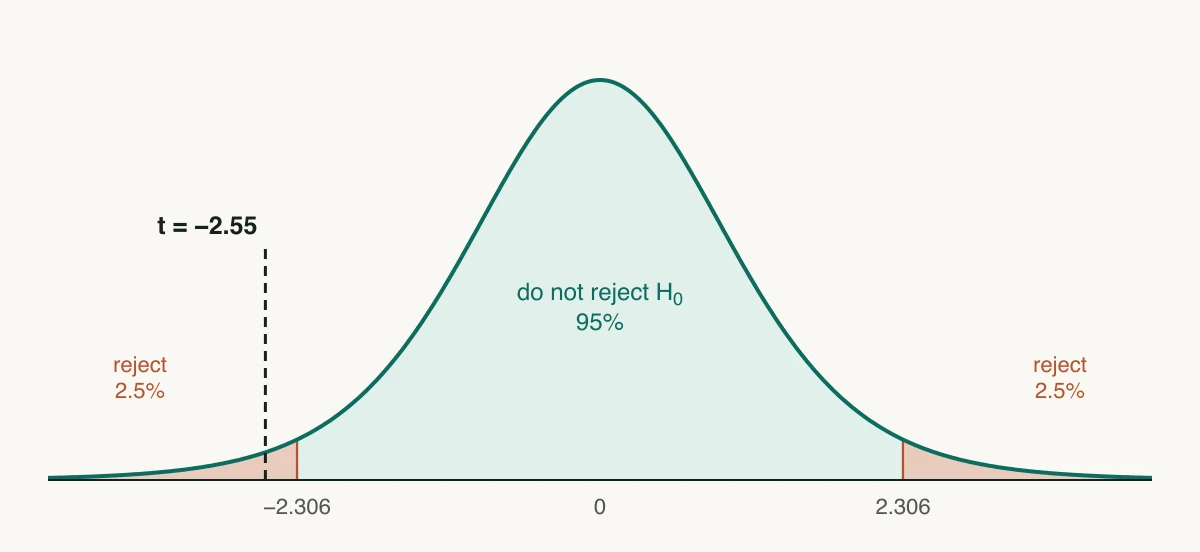
t = (497 − 500) / 1.1785 = −2.5456, with df = 9 − 1 = 8. The sample mean is about 2.5 standard errors below the target.
Step 5: p-value and decision
The two-tailed p-value is 2 · P(T₈ ≤ −2.5456) = 0.0344. The t-table critical value for α = 0.05 with 8 df is 2.306. Because |t| = 2.546 > 2.306, or equivalently p = 0.0344 < 0.05, reject H₀: the mean fill weight differs from 500 g, and the sample points to underfilling.
One-tailed vs two-tailed tests
The alternative hypothesis decides which tail of the t distribution counts as evidence against H₀. The t statistic is the same in all three cases; only the p-value and the critical region change.
| Alternative | Question asked | p-value | Reject H₀ at α = 0.05 when |
|---|---|---|---|
| H₁: μ ≠ 500 | Is the mean fill off target in either direction? | 0.0344 | |t| ≥ 2.306 |
| H₁: μ < 500 | Is the machine underfilling? | 0.0172 | t ≤ −1.860 |
| H₁: μ > 500 | Is the machine overfilling? | 0.9828 | t ≥ 1.860 |
A one-tailed test has more power in the stated direction, but it cannot detect an effect in the other direction at all: the right-tailed p-value of 0.98 shows what happens when the data go the opposite way.
How to know if a test is one-tailed or two-tailed
Read the research question, not the data. If it asks whether the mean is different from, changed from or not equal to μ₀, the test is two-tailed. If it asks whether the mean is less than, below, at most, greater than or exceeds μ₀, and a result in the other direction would lead to the same decision as no effect, it is one-tailed. Fix the direction before collecting the data. If you would act on a difference in either direction, use two tails.
t-test or z-test?
The choice depends on one thing: whether the population standard deviation σ is known. If it is, the standard error σ / √n is a fixed number and the statistic z = (x̄ − μ₀) / (σ / √n) follows the standard normal distribution. If σ is estimated by s, the estimate adds uncertainty of its own, and the t distribution’s heavier tails account for it.
| Sample size n | df | t critical value | z critical value |
|---|---|---|---|
| 5 | 4 | 2.776 | 1.960 |
| 10 | 9 | 2.262 | 1.960 |
| 20 | 19 | 2.093 | 1.960 |
| 30 | 29 | 2.045 | 1.960 |
| 100 | 99 | 1.984 | 1.960 |
Suppose long-run records showed that this filling machine has σ = 3.5 g. Then z = (497 − 500) / (3.5 / √9) = −3 / 1.1667 = −2.571 and the two-tailed p = 0.0101 from the One-Sample Z-Test Calculator. Without that knowledge, reading the t statistic of −2.5456 against the normal curve would give p = 0.0109 where the correct value is 0.0344. With only nine observations, that shortcut makes the p-value about three times too small.
In practice σ is almost never known, so the t-test is the default at every sample size. The old rule “use z when n ≥ 30” only reflects that the two give nearly the same answer for large n.
One-sample vs two-sample t-test, paired t-test and ANOVA
The difference between a one-sample and a two-sample t-test is what the mean is compared with. A one-sample test compares one group with a fixed number; a two-sample test compares two groups with each other, so both means carry sampling error. Choose by the number of groups and how they are related:
| Design | Test | Hypothesis | df |
|---|---|---|---|
| One group vs a fixed value μ₀ | One-sample t-test | μ = μ₀ | n − 1 |
| Two related measurements per subject | Paired t-test | μ_d = 0 | pairs − 1 |
| Two independent groups | Two-sample (independent) t-test | μ₁ = μ₂ | n₁ + n₂ − 2 (pooled) |
| Three or more independent groups | One-way ANOVA | μ₁ = μ₂ = … = μₖ | k − 1 and N − k |
Use a one-way ANOVA instead of t-tests when there are three or more groups. Running every pairwise t-test inflates the chance of at least one false positive: with three groups and three tests at α = 0.05 it rises to as much as 14% (1 − 0.95³). With exactly two groups, ANOVA and the pooled t-test are equivalent (F = t²). For any other design, the test chooser walks through the options.
Confidence interval and effect size
With 8 df and 95% confidence the critical value is 2.306, so the interval is 497 ± 2.306 × 1.1785 = 497 ± 2.72, or 494.28 g to 499.72 g. The target of 500 lies just outside it. That is no coincidence: a two-tailed test at α = 0.05 rejects H₀ exactly when the 95% confidence interval excludes μ₀. The interval is the more informative of the two, because it shows every value of μ the data are compatible with. The Mean Confidence Interval Calculator computes it directly.
Here d = (497 − 500) / 3.5355 = −0.85: the mean fill is 0.85 standard deviations below target, a large standardized effect by Cohen’s benchmarks of 0.2, 0.5 and 0.8. In raw units the shortfall is 3 g, or 0.6% of the label weight. Whether that matters is a question for the quality standard, not for the p-value. The Effect Size Calculator reports d from either raw data or t and n.
Running a one-sample t-test in R, Python, SPSS and Excel
Every major package runs the test from the raw values and the test value μ₀. With the nine cereal weights, each one below returns t = −2.546, df = 8 and p = 0.034.
| Software | Command or menu |
|---|---|
| R | t.test(x, mu = 500); add alternative = "less" for a left-tailed test |
| Python (SciPy) | scipy.stats.ttest_1samp(x, 500); add alternative="less" for a left-tailed test |
| SPSS | Analyze → Compare Means → One-Sample T Test, then enter 500 as the Test Value |
| Excel | No one-sample option in T.TEST. Compute t with the formula above, then =T.DIST.2T(ABS(t), n-1) for the two-tailed p-value |
Reporting and common mistakes
An APA-style sentence gives the sample mean and standard deviation, the test value, then t with its degrees of freedom, p, the effect size and the confidence interval: “The mean fill weight (M = 497.00 g, SD = 3.54) was below the 500 g target, t(8) = −2.55, p = .034, d = −0.85, 95% CI [494.28, 499.72].”
- Taking μ₀ from the data. The test value must be fixed before you look at the sample. Testing against a number suggested by the same data makes the p-value meaningless.
- Using another sample’s mean as μ₀. A mean estimated from a second sample has its own sampling error. Compare the two samples with an independent samples t-test.
- Using z with a small sample and unknown σ. This understates the p-value, as the comparison above shows.
- Ignoring an outlier in a small sample. Plot the data first. One extreme value can either create or hide a significant result.
- Sampling for convenience. Nine consecutive boxes from one minute of production are not a random sample of the shift.
- Stopping at the p-value. Report the confidence interval and effect size too; see What Is a P-Value? Meaning, Calculation and Common Mistakes.
Frequently asked questions
When should I use a one-sample t-test?
What is the difference between a one-sample t-test and a z-test?
What are the degrees of freedom in a one-sample t-test?
How do you calculate the t statistic for a one-sample t-test?
What is the difference between a one-sample and a two-sample t-test?
Can I run a one-sample t-test with a small sample?
How is the one-sample t-test related to a confidence interval?
Is a paired t-test the same as a one-sample t-test?
Further reading
Cite this page
Statculator. (2026, November 14). One-Sample t-Test: Formula, Assumptions and Worked Example. Retrieved November 14, 2026, from https://statculator.com/learn/one-sample-t-test/