Statistical TestsStudy Design & Sample Size
Type I vs Type II Errors (Type 1 vs Type 2): Definitions and Examples
Type 1 vs Type 2 errors (Type I and II): false positives vs false negatives, α, β and power, 10 examples, a worked power calculation and how to reduce each.
By Hira Noor, BS Mathematics · Updated · 14 min read
Summary
Type 1 and Type 2 errors (Type I and Type II errors) are the two ways a hypothesis test can reach the wrong conclusion. A Type I error is a false positive: rejecting a null hypothesis that is true. A Type II error is a false negative: failing to reject a null hypothesis that is false. The probability of a Type I error is the significance level α, the probability of a Type II error is β, and power = 1 − β is the chance of detecting a real effect. For a fixed sample size, lowering one error rate raises the other. Example: convicting an innocent defendant is a Type I error; acquitting a guilty one is a Type II error.
Key takeaways
- Type I error: H₀ is true but you reject it (false positive). Its probability is α, which you choose before the test.
- Type II error: H₀ is false but you fail to reject it (false negative). Its probability is β, and power = 1 − β.
- β is not a single number: it depends on α, the sample size, the variability and how large the true effect is.
- With n fixed, a smaller α means a larger β. Only more data, less noise or a larger effect lowers both.
- Which error is worse depends on what each mistake costs, so set α and the target power case by case.
- Memory aid: a Type I error is a false alarm (crying wolf when there is no wolf); a Type II error is a missed alarm (no one comes when the wolf is real).
On this page
- What are Type I and Type II errors?
- α, β and power
- Type 1 and Type 2 error examples
- How to remember Type 1 and Type 2 errors
- The trade-off between Type I and Type II errors
- Worked example: calculating β and power
- How to reduce each error
- Which error is worse?
- Type I and Type II errors in A/B testing
- Describing Type 1 and Type 2 errors in AP Statistics
- Type III and Type IV errors
- Common misconceptions
- Frequently asked questions
What are Type I and Type II errors?
A hypothesis test ends in one of two decisions: reject the null hypothesis H₀, or fail to reject it. H₀ itself is either true or false, and you never observe which. That gives four possible outcomes, two correct and two wrong. Whether you write Type I vs Type II errors, Type 1 vs Type 2 errors or Type one and Type two errors, the terms mean the same thing in statistics.
| Decision | H₀ is actually true | H₀ is actually false |
|---|---|---|
| Reject H₀ | Type I error (false positive), probability α | Correct decision (true positive), probability 1 − β = power |
| Fail to reject H₀ | Correct decision (true negative), probability 1 − α | Type II error (false negative), probability β |
A Type I error claims an effect that does not exist: the test comes out significant although H₀ is true. A Type II error misses an effect that does exist: the test comes out non-significant although H₀ is false. The numbering comes from Neyman and Pearson, who called them errors of the first and second kind. It does not rank them by seriousness.
Each probability is conditional on a different state of the world: α is calculated assuming H₀ is true, and β assuming H₀ is false. They therefore do not add up to 1. The pairs that do add up to 1 share a column of the table: α with 1 − α, and β with power.
The same table appears outside hypothesis testing under other names. In diagnostic testing and machine learning it is the confusion matrix: the false positive rate (1 − specificity) plays the role of α, and the false negative rate (1 − sensitivity) plays the role of β. A screening test with 95% specificity and 80% sensitivity therefore behaves like a test with α = 0.05 and power 0.80.
| Aspect | Type I error | Type II error |
|---|---|---|
| Also called | False positive, error of the first kind, α error | False negative, error of the second kind, β error |
| What really holds | H₀ is true | H₀ is false |
| Decision made | Reject H₀ | Fail to reject H₀ |
| In plain words | Finding an effect that is not there | Missing an effect that is there |
| Probability | α, the significance level | β; power = 1 − β |
| Who sets it | You choose α before the test | Follows from α, n, variability and the true effect |
| Main way to reduce it | Smaller α, multiple-comparison corrections | Larger sample, less noise, larger effect |
| Courtroom example | An innocent defendant is convicted | A guilty defendant is acquitted |
α, β and power
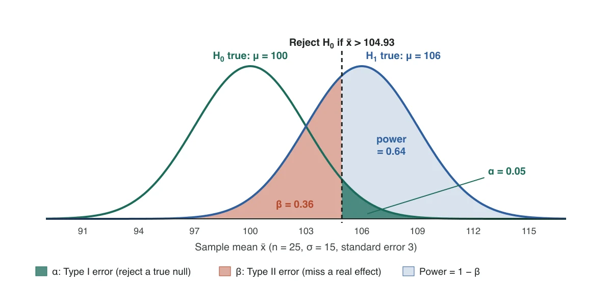
- α, the significance level, is the probability of a Type I error: P(reject H₀ | H₀ true). You choose it before collecting data. The most common value is 0.05, with 0.01 and 0.10 also in use.
- β is the probability of a Type II error: P(fail to reject H₀ | H₀ false). You do not set it directly. It follows from α, the sample size, the variability of the data and how far the truth lies from H₀.
- Power = 1 − β is the probability that the test detects an effect of a given size. Studies are commonly planned for a power of 0.80 or 0.90, which means accepting β = 0.20 or 0.10.
The link to p-values is direct. You reject H₀ when p ≤ α, so when H₀ is true a p-value at or below 0.05 still turns up in 5% of studies, and each of those is a Type I error. The guide What Is a P-Value? Meaning, Calculation and Common Mistakes covers that decision rule in detail.
Type 1 and Type 2 error examples
In any setting, start by writing down H₀. The Type I error is then “acting as if H₀ were false when it is true”, and the Type II error is the reverse.
| Setting | Null hypothesis H₀ | Type I error (false positive) | Type II error (false negative) |
|---|---|---|---|
| Medical screening test | The patient does not have the disease | A healthy patient tests positive and is sent for further tests | A patient with the disease tests negative and goes untreated |
| Criminal trial | The defendant is innocent | An innocent defendant is convicted | A guilty defendant is acquitted |
| A/B test of a new checkout page | The new page converts no better than the old one | The team ships a page that is no better, believing it is | The team discards a page that really is better |
| Clinical drug trial | The drug works no better than placebo | An ineffective drug is approved | An effective drug is abandoned |
| Email spam filter | The email is legitimate | A genuine email lands in the spam folder | A spam email reaches the inbox |
| Smoke alarm | There is no fire | The alarm sounds while someone is cooking | The alarm stays silent during a real fire |
| Factory quality control | The batch meets specification | A good batch is scrapped | A defective batch is shipped to customers |
| Airport security scanner | The bag holds no prohibited item | A harmless bag is pulled for a manual search | A prohibited item passes through |
| Bank fraud detection | The card transaction is genuine | A genuine purchase is declined | A fraudulent purchase goes through |
| Home pregnancy test | The person is not pregnant | The test reads positive for someone who is not pregnant | The test reads negative for someone who is pregnant |
The courtroom shows the asymmetry built into testing. “Innocent until proven guilty” makes innocence the null hypothesis and demands strong evidence before rejecting it, which keeps Type I errors rare at the price of more Type II errors. An acquittal means “not proven guilty”, just as a non-significant result means “fail to reject H₀”, not “H₀ is true”.
The labels depend entirely on how H₀ is stated. In the smoke-alarm row, H₀ is “there is no fire”, so a false alarm is the Type I error. If you reversed the hypotheses, the names of the two errors would swap, which is why the null hypothesis always comes first.
How to remember Type 1 and Type 2 errors
- The boy who cried wolf. Take H₀ as “there is no wolf”. When the villagers first run out for a wolf that is not there, they make a Type I error. When they later ignore the boy and a real wolf attacks, they make a Type II error.
- False alarm, then missed alarm. Type I comes first in the numbering and in the story: an alarm with nothing behind it. Type II is the alarm that should have gone off and did not.
- Link the error to the decision. A Type I error can only happen when you reject H₀; a Type II error can only happen when you fail to reject it. If your test was significant, the only error you can have made is Type I.
- Tie each Greek letter to its error. α (alpha, the first letter) is the Type I error rate; β (beta, the second letter) is the Type II error rate.
The trade-off between Type I and Type II errors
For a fixed sample size, α and β move in opposite directions. Lowering α pushes the critical value further from what H₀ predicts, so real effects also find it harder to clear, and β rises.
Take a right-tailed z-test of H₀: μ = 100 with σ = 15 and n = 25, when the true mean is 106. Changing only α gives:
| α | Reject H₀ when x̄ exceeds | β (Type II error) | Power |
|---|---|---|---|
| 0.10 | 103.84 | 0.2362 | 0.7638 |
| 0.05 | 104.93 | 0.3612 | 0.6388 |
| 0.01 | 106.98 | 0.6279 | 0.3721 |
Moving from α = 0.05 to α = 0.01 makes false positives five times rarer, but the chance of missing this effect climbs from 36% to 63%. The only ways to lower both error rates together are to collect more data, to reduce the noise in the measurements, or to study a larger effect.
Worked example: calculating β and power
Power of a right-tailed z-test
Problem. A training program is claimed to raise test scores above the population mean of 100, where σ = 15. You plan to test H₀: μ = 100 against H₁: μ > 100 at α = 0.05 with n = 25 participants. If the program truly raises the mean to 106, what are β and the power?
- 01Standard error. SE = σ / √n = 15 / √25 = 3.
- 02Rejection rule. The right-tailed critical value at α = 0.05 is z = 1.6449, so H₀ is rejected when x̄ > 100 + 1.6449 × 3 = 104.9346.
- 03Switch to the true distribution. If μ = 106, the sample mean is normal with mean 106 and standard error 3. The cut-off lies (104.9346 − 106) / 3 = −0.3551 standard errors from the true mean.
- 04Power. P(x̄ > 104.9346 | μ = 106) = P(Z > −0.3551) = 0.6388.
- 05Type II error. β = 1 − 0.6388 = 0.3612.
Answer. The test has a 5% chance of a Type I error if the program does nothing, and a 36% chance of a Type II error if it raises the mean by 6 points. Power is about 64%, below the usual 80% target.
The same steps give a general formula for the Type II error of a right-tailed z-test, where Φ is the standard normal cumulative distribution function and z₁₋α is the critical value:
With z₀.₉₅ = 1.6449, μ₁ − μ₀ = 6 and σ / √n = 3, β = Φ(1.6449 − 2) = Φ(−0.3551) = 0.3612, as above. Sample size and effect size change the picture quickly. Keeping α = 0.05 and σ = 15:
| Sample size | True mean 103 (d = 0.2) | True mean 106 (d = 0.4) | True mean 109 (d = 0.6) |
|---|---|---|---|
| n = 25 | 0.2595 | 0.6388 | 0.9123 |
| n = 50 | 0.4088 | 0.8817 | 0.9953 |
| n = 100 | 0.6388 | 0.9907 | > 0.9999 |
Here d is the effect in standard-deviation units, (μ − μ₀) / σ. Reaching 80% power for the 6-point effect takes n = 39, and 90% power takes n = 54. The same logic drives every power analysis. For a two-sided, two-sample t-test at α = 0.05, detecting a medium effect of d = 0.5 with 80% power needs 64 participants per group (63 by the normal-approximation formula), while 30 per group gives only 48% power.
Try it: Sample Size CalculatorChoose α and the power you want, enter the difference you need to detect, and get the sample size for comparing two means or two proportions.How to reduce each error
The two errors respond to different levers.
Reducing Type I errors
- Choose a smaller α, such as 0.01, when a false positive is costly.
- Correct for multiple comparisons. Twenty independent tests at α = 0.05 have a 64% chance of at least one false positive when every null hypothesis is true (1 − 0.95²⁰ = 0.6415). A Bonferroni-type correction, or one overall test such as ANOVA in place of many t-tests, keeps the overall rate at α.
- Fix the analysis before seeing the data. Choosing the outcome, the tail or the stopping point after looking at the results pushes the real false-positive rate above the nominal α.
Reducing Type II errors
- Increase the sample size. The standard error shrinks in proportion to 1/√n, which is the most direct way to raise power. Plan it with the Sample Size Calculator.
- Reduce variability. More precise measurement, a more homogeneous sample or a paired design (see the Paired t-Test Calculator) lowers the noise the effect has to stand out from.
- Study a larger effect where you can, for example a stronger dose or a longer exposure. The Effect Size Calculator converts an expected difference into a standardized effect such as Cohen’s d for planning.
- Use a one-tailed test only when it is justified in advance. It has more power in the predicted direction and none in the other.
- Raise α, accepting more false positives, when a missed effect is the costlier mistake.
Which error is worse?
Neither is worse in general; it depends on what each mistake costs. The convention of α = 0.05 with 80% power sets β = 0.20, four times α, which treats a false positive as the more serious error. That ratio does not suit every problem.
- Type I is usually worse when acting on a false claim is expensive or hard to reverse: approving an ineffective drug, convicting an innocent person, or publishing a finding that others will build on. Use a small α.
- Type II is usually worse when missing a real effect is the bigger loss: a screening test that misses a treatable disease, or a safety check that fails to notice a defect. Accept a larger α, or pay for a larger sample, to gain power.
- In low-stakes, reversible decisions, such as an A/B test of a button colour, both errors are cheap and a looser α such as 0.10 can be reasonable.
Type I and Type II errors in A/B testing
An A/B test is a hypothesis test with H₀ “the variant performs no better than the control”. A Type I error ships a change that does nothing, and a Type II error throws away a change that works. Two habits make each error far more common than the nominal rates suggest.
- Peeking inflates Type I errors. Checking the results repeatedly and stopping as soon as p < 0.05 is not a test at α = 0.05. With 5 equally spaced looks the overall false-positive rate is about 14%, and with 10 looks about 19%. Fix the sample size in advance, or use a sequential method designed for repeated looks.
- Small tests produce Type II errors. Detecting a lift in conversion rate from 10% to 12% at α = 0.05 (two-sided) with 80% power takes about 3,841 visitors per variant. With 1,000 per variant the power is only about 30%, so the test misses a real 2-point lift 70% of the time. Work out the size first with the Sample Size Calculator.
- Low-power wins are often exaggerated. When an underpowered test does reach significance, the observed lift tends to overstate the true one, a Type M error in the terms used below.
Describing Type 1 and Type 2 errors in AP Statistics
AP Statistics questions usually ask you to describe an error “in context” and to give a consequence. A definition alone (“rejecting a true null hypothesis”) does not earn credit; the answer has to name the parameter, the claim and the decision in the words of the problem.
- Write H₀ in context and decide whether the error you are asked about rejects it (Type I) or fails to reject it (Type II).
- State what is actually true and what you concluded. Type I: “H₀ is true, but we concluded H₁.” Type II: “H₁ is true, but we did not find convincing evidence for it.”
- Add a consequence that follows from acting on the wrong conclusion.
AP-style example: a battery claim
Problem. A manufacturer claims its batteries last 40 hours on average. A consumer group tests H₀: μ = 40 against Hₐ: μ < 40, where μ is the mean life of all the manufacturer’s batteries. Describe a Type I and a Type II error in context, with a consequence of each.
- 01Type I error. The mean life of all the batteries really is 40 hours, but the group finds convincing evidence that it is less than 40. Consequence: the group publishes a false complaint and damages an honest manufacturer.
- 02Type II error. The mean life of all the batteries really is less than 40 hours, but the group does not find convincing evidence of it. Consequence: consumers keep buying batteries that fall short of the advertised life.
Answer. Each answer names the parameter (mean life of all batteries), the truth, the conclusion and a consequence. Writing “fail to find convincing evidence” rather than “accept H₀” keeps the wording correct.
Type III and Type IV errors
Only Type I and Type II errors are part of the Neyman–Pearson theory of testing. Later authors proposed further “types”, and their definitions are not standardized, so check which meaning a source intends.
| Term | Usual meaning | Example |
|---|---|---|
| Type III error | Correctly rejecting H₀ for the wrong reason (Mosteller, 1948), concluding the wrong direction after a two-sided test (Kaiser, 1966), or giving the right answer to the wrong problem (Kimball, 1957) | A two-sided test is significant and the report says the drug raised blood pressure when it lowered it |
| Type IV error | Misinterpreting a correctly rejected hypothesis, such as choosing the wrong follow-up test (Marascuilo and Levin, 1970) | An ANOVA rejects H₀ but the wrong pair of groups is named as different |
| Type S and Type M errors | Getting the sign (S) or the magnitude (M) of an effect wrong, an idea from Gelman and Carlin (2014) for low-power studies | A small study reports a large effect that is mostly noise |
Common misconceptions
- “α is the probability that a significant result is a false positive.” α is the probability of rejecting H₀ when H₀ is true. The share of significant results that are false positives also depends on how often the tested hypotheses are true and on the power of the studies.
- “α + β = 1.” They are conditional on different states of the world. In the worked example α = 0.05 and β = 0.3612.
- “A non-significant result means there is no effect.” It may be a Type II error. With 30 per group and a medium effect, a t-test misses the effect more often than it finds it.
- “A very small α makes a test safer.” It makes Type I errors rarer and Type II errors more common, unless the sample grows to compensate.
- “The data show which error was made.” They cannot. A single study never reveals whether H₀ is true; the error rates describe how the procedure performs over many studies.
- “Power can be worked out afterwards from the observed effect.” Power computed from the observed effect only restates the p-value. Power is a planning tool, calculated for an effect size chosen before the study.
Frequently asked questions
What is an example of a Type 1 and a Type 2 error?
What is the difference between a Type I and a Type II error?
What is the probability of a Type I error?
How are β and power related?
Does increasing the sample size reduce both types of error?
Is a Type I or a Type II error worse?
How can I remember which error is which?
What are Type 1, 2 and 3 errors?
What is a Type 4 error?
Further reading
- OpenStax, Introductory Statistics 2e, section 9.2: Outcomes and the Type I and Type II Errors
- NIST/SEMATECH e-Handbook of Statistical Methods, section 7.1.3: What are statistical tests?
- Banerjee A. et al. (2009). Hypothesis testing, type I and type II errors. Industrial Psychiatry Journal 18(2)
- Neyman J. and Pearson E. S. (1933). On the problem of the most efficient tests of statistical hypotheses. Philosophical Transactions of the Royal Society A 231
- Gelman A. and Carlin J. (2014). Beyond power calculations: assessing Type S (sign) and Type M (magnitude) errors. Perspectives on Psychological Science 9(6)
Cite this page
Statculator. (2026, November 14). Type I vs Type II Errors (Type 1 vs Type 2): Definitions and Examples. Retrieved November 14, 2026, from https://statculator.com/learn/type-i-vs-type-ii-errors/