Statistical TestsStatistical Tables & Critical Values
One-Way ANOVA: Definition, Formulas and a Worked Example by Hand
Learn one-way ANOVA: what it tests, the null hypothesis, the 3 assumptions, the formulas, a worked example by hand, the ANOVA table and how to report F.
By Hira Noor, BS Mathematics · Updated · 14 min read
Summary
A one-way ANOVA (analysis of variance), also called a one-factor or single-factor ANOVA, tests whether three or more independent groups share the same population mean. It splits the total variability in the data into variation between the group means and variation within the groups, then compares the two with the F statistic, F = MSB / MSW. A large F with a p-value below α means at least one group mean differs; post-hoc tests then show which.
Key takeaways
- The null hypothesis of a one-way ANOVA is that all group means are equal; H₁ says at least one mean differs.
- F = MSB / MSW, with k − 1 and N − k degrees of freedom.
- SST = SSB + SSW, and η² = SSB / SST measures the effect size.
- A significant F says some means differ; Tukey’s HSD shows which pairs.
- Use Welch’s ANOVA for unequal variances and Kruskal–Wallis for ordinal or strongly non-normal data.
On this page
- What is a one-way ANOVA test?
- When to use a one-way ANOVA
- The 3 assumptions of one-way ANOVA
- One-way ANOVA formulas
- One-way ANOVA example worked by hand
- Reading the ANOVA table
- ANOVA from summary statistics
- Effect size and post-hoc tests
- How to report a one-way ANOVA
- One-way ANOVA in R, Python, SPSS and Excel
- One-way vs two-way ANOVA
- When the assumptions fail
- Frequently asked questions
What is a one-way ANOVA test?
One-way analysis of variance compares the means of k independent groups defined by a single factor, such as three teaching methods or four fertilizers. "One-way" means one factor: a single categorical independent variable whose categories (levels) are the groups, and one numeric dependent variable measured on every subject. You will also see it called a one-factor ANOVA test, an ANOVA single factor analysis (the name Excel uses) or a between-subjects one-way ANOVA, because each subject belongs to exactly one group. Despite the name, the question is about means. ANOVA answers it by comparing two different estimates of variance.
Put simply: if the groups really have the same mean, the group averages should differ from each other only about as much as individual values differ inside each group. ANOVA measures both kinds of spread and asks whether the gap between the groups is too large to be chance.
Null hypothesis of one-way ANOVA
The null hypothesis says every group comes from a population with the same mean. The alternative is not that all the means differ, only that at least one does:
The logic is a ratio. If H₀ is true, the group means differ only through random sampling noise, so the variance estimated from the spread of the group means should be about the same size as the variance estimated from inside the groups. If some population means really differ, the between-group estimate is inflated and the ratio F climbs above 1.
Why use an ANOVA instead of several t-tests?
With k groups there are k(k − 1)/2 pairs of means, and each t-test carries its own α chance of a false positive, so the overall error rate grows quickly: with three groups and three tests at α = 0.05, the chance of at least one false positive rises to as much as 14% (1 − 0.95³). ANOVA tests all the means in a single step at one α, and post-hoc procedures then control the error rate across the pairwise comparisons. With exactly two groups the two approaches agree, so the independent samples t-test is the usual choice there.
When to use a one-way ANOVA
Use it when the outcome is a numeric measurement, there is one categorical factor with three or more levels, and every subject appears in only one group. Typical questions:
- Experiments. Does mean plant growth differ between three fertilizers, or mean recovery time between four doses of a drug?
- Education. Do students taught by three different methods have different mean exam scores?
- Business. Does mean customer satisfaction differ between store layouts, regions or ad versions?
- Manufacturing. Do several machines or suppliers produce parts with the same mean strength or diameter?
If the same subjects are measured under every condition, use repeated-measures ANOVA instead. If there are two factors, such as fertilizer and watering schedule, use a two-way ANOVA.
Try it: ANOVA CalculatorHave your groups ready? Paste the values to get the ANOVA table, F, the p-value and η² with every step shown.The 3 assumptions of one-way ANOVA
The F-test is exact when three conditions hold. They are about the populations and the design, so check them before trusting the p-value:
- Independence. Observations are independent within and across groups. This comes from the design, usually random sampling or random assignment, and cannot be repaired afterwards.
- Normality. Each population is approximately normal. ANOVA is fairly robust to mild non-normality, especially with equal group sizes of about 15 or more. Check the residuals (each value minus its group mean) with a histogram or normal probability plot.
- Equal variances. The populations share one variance. A common rule of thumb is that the largest group standard deviation should be no more than about twice the smallest; Levene’s test checks this formally.
For the fertilizer data in the worked example below, the group standard deviations are 2.24, 1.58 and 1.58 cm, a largest-to-smallest ratio of 1.41, and Levene’s test gives F(2, 12) = 0.25 with p = 0.78, so there is no sign of unequal variances.
One-way ANOVA formulas
Let k be the number of groups, nᵢ the size of group i, N = Σnᵢ the total sample size, xᵢⱼ the j-th value in group i, x̄ᵢ the mean of group i, sᵢ its standard deviation, and x̄ the grand mean of all N values.
The p-value is the right-tail area of the F distribution with (k − 1, N − k) degrees of freedom beyond the observed F. Some textbooks call SSB the treatment sum of squares (SSTr) and SSW the error sum of squares (SSE); the formulas are identical.
| Source | SS | df | MS | F |
|---|---|---|---|---|
| Between groups (treatment) | SSB = Σ nᵢ (x̄ᵢ − x̄)² | k − 1 | MSB = SSB / (k − 1) | MSB / MSW |
| Within groups (error) | SSW = Σ (nᵢ − 1) sᵢ² | N − k | MSW = SSW / (N − k) | |
| Total | SST = SSB + SSW | N − 1 |
One-way ANOVA example worked by hand
A horticulture class grows seedlings with three fertilizers, A, B and C, five plants per fertilizer, and records the growth in centimetres after four weeks. Test at α = 0.05 whether mean growth differs by fertilizer.
| Fertilizer | Growth values | nᵢ | Sum | Mean x̄ᵢ |
|---|---|---|---|---|
| A | 2, 5, 6, 4, 8 | 5 | 25 | 5 |
| B | 9, 8, 11, 10, 7 | 5 | 45 | 9 |
| C | 7, 6, 9, 5, 8 | 5 | 35 | 7 |
| All | 15 values | 15 | 105 | 7 |
Step 1: Group means and grand mean
The group means are 25/5 = 5 for A, 45/5 = 9 for B and 35/5 = 7 for C. The grand mean is x̄ = 105/15 = 7. Because the groups are the same size, it also equals the average of the three group means.
Step 2: Between-group sum of squares
SSB = 5(5 − 7)² + 5(9 − 7)² + 5(7 − 7)² = 5(4) + 5(4) + 5(0) = 40.
Step 3: Within-group sum of squares
Square each value’s deviation from its own group mean and add them up:
- A (mean 5): (−3)² + 0² + 1² + (−1)² + 3² = 9 + 0 + 1 + 1 + 9 = 20
- B (mean 9): 0² + (−1)² + 2² + 1² + (−2)² = 0 + 1 + 4 + 1 + 4 = 10
- C (mean 7): 0² + (−1)² + 2² + (−2)² + 1² = 0 + 1 + 4 + 4 + 1 = 10
SSW = 20 + 10 + 10 = 40. As a check, the squared deviations of all 15 values from the grand mean of 7 total 40 for A, 30 for B and 10 for C, so SST = 80, which equals SSB + SSW = 40 + 40.
Step 4: Degrees of freedom, mean squares and F
df_between = 3 − 1 = 2 and df_within = 15 − 3 = 12. Then MSB = 40 / 2 = 20 and MSW = 40 / 12 = 3.3333, so F = 20 / 3.3333 = 6.00.
Step 5: p-value and decision
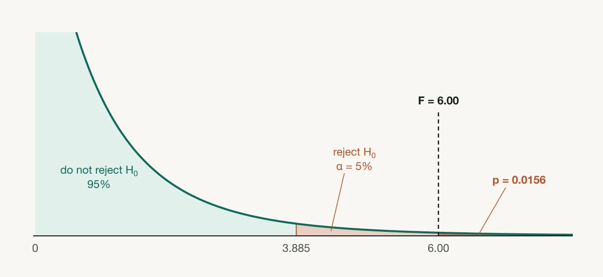
The p-value is P(F ≥ 6.00) for an F distribution with 2 and 12 degrees of freedom, which is 0.0156. The F-table critical value for α = 0.05 and df = (2, 12) is 3.885. Because F = 6.00 > 3.885, or equivalently p = 0.0156 < 0.05, reject H₀: mean growth is not the same for all three fertilizers. Statistical software, for example SciPy’s f_oneway, returns the same F = 6.0 and p = 0.015625.
Reading the ANOVA table
Software and textbooks summarize the calculation in a standard table, with one row per source of variation.
| Source | SS | df | MS | F | p |
|---|---|---|---|---|---|
| Between groups | 40 | 2 | 20.0000 | 6.00 | 0.0156 |
| Within groups (error) | 40 | 12 | 3.3333 | ||
| Total | 80 | 14 |
Two checks catch most arithmetic slips: the SS column adds up (40 + 40 = 80) and so does the df column (2 + 12 = 14). Mean squares are not additive, so the MS column has no total. MSW = 3.3333 is the pooled estimate of the common variance σ², and its square root, 1.8257 cm, is the pooled standard deviation.
ANOVA from summary statistics
If you only have each group’s size, mean and standard deviation, you can still run the test, because SSW = Σ(nᵢ − 1)sᵢ² and SSB needs only the means. The groups do not have to be the same size.
Three store layouts
Problem. Customer satisfaction scores (0–100) are collected under three store layouts. Layout 1: n = 12, x̄ = 71, s = 6. Layout 2: n = 12, x̄ = 79, s = 7. Layout 3: n = 16, x̄ = 75, s = 8. Do the mean scores differ at α = 0.05?
- 01Grand mean, weighted by group size: x̄ = (12 × 71 + 12 × 79 + 16 × 75) / 40 = 3000 / 40 = 75.
- 02SSB = 12(71 − 75)² + 12(79 − 75)² + 16(75 − 75)² = 192 + 192 + 0 = 384.
- 03SSW = 11(6²) + 11(7²) + 15(8²) = 396 + 539 + 960 = 1895.
- 04Degrees of freedom: k − 1 = 2 and N − k = 37. MSB = 384 / 2 = 192 and MSW = 1895 / 37 = 51.2162.
- 05F = 192 / 51.2162 = 3.7488, giving p = 0.0329. The critical value at α = 0.05 with df = (2, 37) is 3.252.
Answer. Because p = 0.0329 < 0.05, reject H₀: at least one layout has a different mean satisfaction score. The effect size is η² = 384 / (384 + 1895) = 0.1685.
Effect size and post-hoc tests
The p-value says whether the means differ; eta squared says by how much, as the share of the total variability that is explained by group membership.
In the fertilizer example η² = 40 / 80 = 0.50: half the variation in growth is associated with fertilizer. η² overstates the population effect in small samples; omega squared corrects for this and gives ω² = (40 − 2 × 3.3333) / (80 + 3.3333) = 0.40. Cohen’s widely quoted benchmarks for η² are about 0.01 (small), 0.06 (medium) and 0.14 (large), but the context of the study matters more than the label.
Tukey’s HSD
A significant F does not say which groups differ. Tukey’s honestly significant difference (HSD) compares every pair of means while holding the family-wise error rate at α. It uses the studentized range distribution q, and with equal group sizes two means differ significantly when their difference exceeds the HSD:
For the fertilizer data, q(0.05; 3, 12) = 3.773 and √(3.3333 / 5) = 0.8165, so HSD = 3.081 cm. Only B − A = 4 exceeds it (adjusted p = 0.012); C − A = 2 and B − C = 2 do not (adjusted p = 0.234 each). Fertilizer B therefore outperforms A, while C cannot be distinguished from either. With unequal group sizes, the Tukey–Kramer version replaces √(MSW / n) with √[(MSW / 2)(1/nᵢ + 1/nⱼ)].
Other follow-up methods include Bonferroni-adjusted t-tests (simple but conservative), Scheffé’s method (for complex contrasts) and Dunnett’s test (for comparing several treatments with a single control).
How to report a one-way ANOVA
Give the F statistic with both degrees of freedom, the p-value and an effect size, then the follow-up comparisons and the group means. In APA style the fertilizer result reads:
If Levene’s test or the standard deviations suggest unequal variances, report Welch’s F with its fractional denominator df instead, for example F(2, 7.84) = 5.16, p = .037.
One-way ANOVA in R, Python, SPSS and Excel
Each package below, given the 15 growth values and a column naming each plant’s fertilizer, returns F = 6.00 with df = (2, 12) and p = 0.0156.
| Software | Command or menu | Follow-up |
|---|---|---|
| R | summary(aov(growth ~ fertilizer, data = d)) | TukeyHSD(aov(...)); oneway.test(growth ~ fertilizer, data = d) for Welch |
| Python (SciPy) | scipy.stats.f_oneway(a, b, c) | scipy.stats.tukey_hsd(a, b, c) |
| SPSS | Analyze → Compare Means → One-Way ANOVA | Post Hoc → Tukey; Options → Welch and homogeneity of variance test |
| Excel | Data → Data Analysis → Anova: Single Factor (Analysis ToolPak) | Output includes the F crit value, 3.885 here |
The output is the same ANOVA table under different labels. The between-groups row may be named after the factor (R), "Between Groups" (SPSS, Excel) or "Treatment"; the within-groups row may be "Residuals" (R), "Within Groups" (SPSS, Excel) or "Error". The p-value appears as Pr(>F) in R, Sig. in SPSS and P-value in Excel. SPSS shows p = .016 as "Sig. .016" and very small p-values as ".000", which should be reported as p < .001.
One-way vs two-way ANOVA
The difference is the number of factors. A one-way ANOVA has one factor and tests one null hypothesis about its group means. A two-way ANOVA has two factors, such as fertilizer and watering schedule, and tests three: the main effect of each factor and their interaction. Choose two-way when a second factor may explain part of the variation or change the effect of the first. The one-way vs two-way ANOVA guide compares them side by side.
When the assumptions fail
| Problem | Alternative | What changes |
|---|---|---|
| Unequal variances | Welch’s ANOVA | Weights each group by nᵢ / sᵢ² and adjusts the denominator df; follow up with Games–Howell comparisons |
| Ordinal outcome, or strong skew and outliers in small groups | Kruskal–Wallis H test | Ranks all N values and compares the groups’ mean ranks; follow up with Dunn’s test |
| Right-skewed positive data such as times or incomes | Log or square-root transformation, then ANOVA | Means are compared on the transformed scale |
| The same subjects measured under every condition | Repeated-measures ANOVA or the Friedman test | Accounts for the pairing that one-way ANOVA would ignore |
Applied to the fertilizer data, Welch’s ANOVA gives F = 5.16 with df = (2, 7.84) and p = 0.037, and the Kruskal–Wallis test gives H = 6.96 with p = 0.031 after the correction for ties. All three methods reject H₀ at α = 0.05 here. When they disagree, report the method whose assumptions your data meet.
With exactly two groups, one-way ANOVA is equivalent to the pooled two-sample t-test (F = t²), and Welch’s ANOVA is equivalent to Welch’s t-test.
Frequently asked questions
What is the null hypothesis for a one-way ANOVA?
What does the F statistic mean in ANOVA?
What is the difference between one-way and two-way ANOVA?
Can I use ANOVA with only two groups?
What should I do after a significant ANOVA?
Do the groups need equal sample sizes?
How do I find the critical F value for ANOVA?
Further reading
Cite this page
Statculator. (2026, November 14). One-Way ANOVA: Definition, Formulas and a Worked Example by Hand. Retrieved November 14, 2026, from https://statculator.com/learn/one-way-anova/