Two-Way ANOVA: Main Effects, Interaction and a Worked Example
Two-way ANOVA (two-way analysis of variance) explained: main effects, interaction, the formula, a worked example with its ANOVA table, reporting and software.
By Hira Noor, BS Mathematics · Updated · 15 min read
Summary
Two-way ANOVA (two-way analysis of variance) tests how two categorical factors affect one numeric outcome. It splits the total variation into four parts: factor A, factor B, the A × B interaction and error. Dividing each of the first three mean squares by the error mean square gives three F tests: two main effects and one interaction. A significant interaction means the effect of one factor depends on the level of the other. Use it when every observation belongs to one level of each factor and the subjects are independent.
Key takeaways
- Two factors give three null hypotheses: no main effect of A, no main effect of B and no A × B interaction.
- In a balanced design SST = SSA + SSB + SSAB + SSE, and each effect has F = MS(effect) / MSE.
- Degrees of freedom: a − 1 for A, b − 1 for B, (a − 1)(b − 1) for the interaction and ab(n − 1) for error.
- Read the interaction first. If it is significant, follow up with simple effects instead of relying on the main effects.
- Testing the interaction requires at least two observations in every cell.
- Report each effect as F(df effect, df error) with its p-value and an effect size such as partial η².
On this page
- What two-way ANOVA tests
- Why use a two-way ANOVA?
- The model and the three hypotheses
- Two-way ANOVA formula: sums of squares, df and F
- Worked example by hand
- The two-way ANOVA table
- Interpreting the interaction, and what to do next
- Effect size and how to report a two-way ANOVA
- How to run a two-way ANOVA in R, Python, Excel and SPSS
- Assumptions
- With and without replication
- Two-way vs factorial, mixed and repeated-measures ANOVA
- Frequently asked questions
What two-way ANOVA tests
Two-way analysis of variance analyses one numeric outcome measured under every combination of two categorical factors. Factor A has a levels and factor B has b levels, so the design has a × b cells. One analysis answers three questions:
- Main effect of A. Averaged over the levels of B, do the means differ across the levels of A?
- Main effect of B. Averaged over the levels of A, do the means differ across the levels of B?
- Interaction A × B. Does the effect of A depend on the level of B?
Take seedlings grown with two fertilizers (factor A) under three watering schedules (factor B). With no interaction, switching fertilizer changes growth by the same amount at every watering level. With an interaction, the size of the fertilizer effect, or even its direction, changes from one watering level to another.
Two separate one-way ANOVAs cannot test the interaction, and each leaves the other factor’s variation in its error term. One-Way vs Two-Way ANOVA: Differences and When to Use Each compares the two approaches on the same data.
Why use a two-way ANOVA?
- It tests the interaction. Only a design that crosses both factors can show whether the effect of one depends on the other. Separate one-way analyses never can.
- It has more power. Variation explained by the second factor is removed from the error term. In the worked example below, a one-way ANOVA on watering alone gives F(2, 15) = 5.19, p = 0.019; the two-way analysis of the same 18 values gives F(2, 12) = 18.00, p = 0.0002.
- It uses every observation twice. Each seedling counts towards the fertilizer comparison and the watering comparison, so one experiment answers questions that would otherwise need two.
- It controls a nuisance variable. When the second factor is a block (a field, a batch, a day), including it keeps that variation out of the treatment comparison.
Choose a one-way ANOVA instead when there is only one grouping factor, and a repeated-measures or mixed design when the same subjects appear in more than one cell.
The model and the three hypotheses
μ is the overall mean, αᵢ is the effect of level i of factor A, βⱼ is the effect of level j of factor B, (αβ)ᵢⱼ is the interaction effect belonging to that cell alone, and εᵢⱼₖ is random error, assumed normal with mean 0 and the same variance in every cell.
Each null hypothesis gets its own F test; each alternative says that at least one of those effects is not zero.
Two-way ANOVA formula: sums of squares, df and F
The formulas below are for a balanced design: n observations in each cell and N = abn in total. Write x̄ᵢⱼ for a cell mean, x̄ᵢ· for the mean of row i (level i of A, over all of B), x̄·ⱼ for the mean of column j, and x̄ for the grand mean.
The interaction term measures how far each cell mean sits from the value predicted by adding its row effect and column effect to the grand mean. Each F is referred to an F distribution with the effect’s df in the numerator and the error df in the denominator. These ratios assume fixed factors, meaning the levels were chosen deliberately; random factors change the denominators.
Worked example by hand
A horticulture class crosses two fertilizers (standard, enriched) with three watering schedules (low, medium, high). Three seedlings are grown under each of the six combinations, 18 in all, and growth after four weeks is recorded in centimetres. Test the three effects at α = 0.05. Here a = 2, b = 3 and n = 3.
| Fertilizer | Low water | Medium water | High water | Row mean |
|---|---|---|---|---|
| Standard | 4, 5, 6 (mean 5) | 4, 6, 8 (mean 6) | 6, 6, 9 (mean 7) | 6 |
| Enriched | 3, 6, 6 (mean 5) | 8, 10, 12 (mean 10) | 14, 14, 17 (mean 15) | 10 |
| Column mean | 5 | 8 | 11 | Grand mean 8 |
Step 1: Main-effect sums of squares
Each row mean is based on b·n = 9 seedlings and each column mean on a·n = 6. SSA = 9 × [(6 − 8)² + (10 − 8)²] = 9 × 8 = 72. SSB = 6 × [(5 − 8)² + (8 − 8)² + (11 − 8)²] = 6 × 18 = 108.
Step 2: Interaction sum of squares
For every cell compute cell mean − row mean − column mean + grand mean:
- Standard: 5 − 6 − 5 + 8 = 2, then 6 − 6 − 8 + 8 = 0, then 7 − 6 − 11 + 8 = −2.
- Enriched: 5 − 10 − 5 + 8 = −2, then 10 − 10 − 8 + 8 = 0, then 15 − 10 − 11 + 8 = 2.
SSAB = 3 × (4 + 0 + 4 + 4 + 0 + 4) = 3 × 16 = 48.
Step 3: Error sum of squares
Add the squared deviations of each value from its own cell mean. The six cells give 2, 8 and 6 for the standard row (for example (4 − 5)² + (5 − 5)² + (6 − 5)² = 2) and 6, 8 and 6 for the enriched row, so SSE = 2 + 8 + 6 + 6 + 8 + 6 = 36.
Check with the total: the 18 values sum to 144 and their squares sum to 1416, so SST = 1416 − 144² / 18 = 1416 − 1152 = 264, which equals 72 + 108 + 48 + 36.
Step 4: Degrees of freedom, mean squares and F
df(A) = 1, df(B) = 2, df(AB) = 1 × 2 = 2 and df(error) = 2 × 3 × (3 − 1) = 12. The mean squares are MSA = 72, MSB = 108 / 2 = 54, MSAB = 48 / 2 = 24 and MSE = 36 / 12 = 3. So F(A) = 72 / 3 = 24.00, F(B) = 54 / 3 = 18.00 and F(AB) = 24 / 3 = 8.00.
Step 5: p-values and decisions
From the F-table, the α = 0.05 critical values are 4.747 for df = (1, 12) and 3.885 for df = (2, 12). All three F statistics exceed them: p = 0.0004 for fertilizer, p = 0.0002 for watering and p = 0.0062 for the interaction. Reject all three null hypotheses.
The two-way ANOVA table
| Source | SS | df | MS | F | p |
|---|---|---|---|---|---|
| Fertilizer (A) | 72 | 1 | 72 | 24.00 | 0.0004 |
| Watering (B) | 108 | 2 | 54 | 18.00 | 0.0002 |
| Fertilizer × Watering | 48 | 2 | 24 | 8.00 | 0.0062 |
| Error (within cells) | 36 | 12 | 3 | ||
| Total | 264 | 17 |
The SS column and the df column each add up to their totals (1 + 2 + 2 + 12 = 17). MSE = 3 is the pooled within-cell variance, so the pooled standard deviation is √3 = 1.73 cm. Because the design is balanced, Type I, II and III sums of squares coincide and any statistics package returns this same table.
Statculator does not have a two-way ANOVA calculator yet. You can still check most of the arithmetic with the one-way tool: entered as six separate groups, the cells give a between-groups SS of 228 = 72 + 108 + 48 and a within-groups SS of 36, the SSE above.
Try it: ANOVA CalculatorOne-way only: enter the six cells as six groups to confirm SSE = 36 and MSE = 3, then split the between-groups SS of 228 by hand.Interpreting the interaction, and what to do next
Read the interaction row first. A main effect is an average over the other factor, and when the factors interact that average may describe no single condition well.
An interaction plot shows the pattern. Put the watering levels on the horizontal axis and mean growth on the vertical axis, then draw one line per fertilizer through its three cell means. For these data the standard-fertilizer line rises gently from 5 to 6 to 7 cm, while the enriched line climbs from 5 to 10 to 15 cm. The lines start at the same point and fan apart. Parallel lines would mean no interaction; lines that diverge, converge or cross signal one.
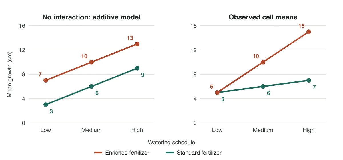
In words: the enriched fertilizer adds nothing under low watering, 4 cm under medium watering and 8 cm under high watering. The fertilizer main effect, 10 − 6 = 4 cm, is the average of those three gaps. It overstates the benefit for dry conditions and understates it for wet ones.
Simple effects
A simple effect is the effect of one factor at a single level of the other. Its sum of squares is n times the squared deviations of the relevant cell means from their own mean, for example 3 × [(6 − 8)² + (10 − 8)²] = 24 at medium watering, and it is tested against the same MSE.
| Watering | Enriched − standard | SS | F | p |
|---|---|---|---|---|
| Low | 5 − 5 = 0 cm | 0 | 0.00 | 1.0000 |
| Medium | 10 − 6 = 4 cm | 24 | 8.00 | 0.0152 |
| High | 15 − 7 = 8 cm | 96 | 32.00 | 0.0001 |
The three sums of squares total 120 = SSA + SSAB: simple effects repackage the main effect and the interaction. With three tests, a Bonferroni correction compares each p-value with 0.05 / 3 = 0.0167, and the medium and high comparisons still pass. The P-Value from F Calculator converts any of these F values.
Post-hoc comparisons
When the interaction is not significant, interpret the main effects directly. A two-level factor needs no follow-up. For a factor with three or more levels, compare its marginal means with Tukey’s HSD, using MSE and the error df as in the one-way ANOVA guide. When the interaction is significant, compare cell means within each simple effect instead.
Effect size and how to report a two-way ANOVA
Partial eta squared is the effect size most software reports for factorial designs. For the seedling data it is 72 / 108 = 0.667 for fertilizer, 108 / 144 = 0.750 for watering and 48 / 84 = 0.571 for the interaction. Partial values for different effects can add up to more than 1, because each uses its own denominator. Plain eta squared divides by SST = 264 instead (0.27, 0.41 and 0.18) and does add up, together with SSE / SST = 0.14, to 1. Say which one you report.
How to run a two-way ANOVA in R, Python, Excel and SPSS
Put the data in long format, one row per observation with a column for each factor and one for the outcome (Excel’s ToolPak is the exception). With the seedling data each of these reproduces the table above: F = 24.00, 18.00 and 8.00.
| Software | Command | Notes |
|---|---|---|
| R | summary(aov(growth ~ fertilizer * water, data = df)) | a * b expands to both main effects plus the a:b interaction. aov uses sequential (Type I) sums of squares, which only match Type II and III when the design is balanced. |
| Python (statsmodels) | anova_lm(ols("growth ~ C(fertilizer) * C(water)", data=df).fit(), typ=2) | Import ols from statsmodels.formula.api and anova_lm from statsmodels.stats.anova. typ sets the sum-of-squares type. |
| Excel | Data → Data Analysis → Anova: Two-Factor With Replication | Lay out one block of rows per level of A with a label column, and set “Rows per sample” to n (3 here). Excel labels the rows Sample, Columns, Interaction and Within. |
| SPSS | Analyze → General Linear Model → Univariate | Enter the outcome as the dependent variable and both factors as fixed factors. SPSS uses Type III sums of squares by default. |
Assumptions
- Independence. Each observation comes from a different, unrelated unit, ideally assigned to its cell at random. Measuring the same subjects in several cells requires a repeated-measures or mixed design.
- Normal errors. Within each cell the values are approximately normal. Check the residuals (each value minus its cell mean) with a histogram or the Shapiro–Wilk test.
- Equal variances. All ab cells share one variance. Compare the cell standard deviations or run Levene’s test across the cells.
In the seedling data the six cell standard deviations run from 1.00 to 2.00 cm, and Levene’s test across the six cells (median-centred) gives p = 0.99, so equal variances are reasonable. A Shapiro–Wilk test of the 18 residuals gives p = 0.037, which mostly reflects the many tied values in small whole-number data; a balanced design with equal cell sizes is fairly robust to mild non-normality.
If the assumptions fail: a log or square-root transformation often fixes right-skewed outcomes whose spread grows with the mean. Unequal variances in a balanced design matter less than in an unbalanced one; with unequal cell sizes as well, use heteroscedasticity-consistent (robust) standard errors in software. For ordinal or badly skewed data, a rank-based method such as the aligned rank transform keeps the interaction test, whereas the Kruskal–Wallis test handles only one factor.
With and without replication
Replication means more than one observation per cell. It supplies a within-cell error term that is separate from the interaction. Excel’s Analysis ToolPak lists the two versions as “Anova: Two-Factor With Replication” and “Anova: Two-Factor Without Replication”.
| Feature | With replication (n ≥ 2 per cell) | Without replication (n = 1 per cell) |
|---|---|---|
| Observations | a × b × n | a × b |
| Interaction test | Yes: F(AB) = MSAB / MSE | No: interaction cannot be separated from error |
| Error term | Within-cell variation, df = ab(n − 1) | Residual (interaction) variation, df = (a − 1)(b − 1) |
| Extra assumption | None | The factors do not interact (additivity) |
| Typical use | Factorial experiments | Randomized block designs, where one factor is a blocking variable |
The example shows the cost of a single observation per cell. Had only the six cell means been recorded, SSA = 24 and SSB = 36 would be tested against a residual SS of 16 with 2 df, giving F = 3.00 (p = 0.23) and F = 2.25 (p = 0.31). The real interaction would count as noise and neither main effect would be detected.
Two-way vs factorial, mixed and repeated-measures ANOVA
These names overlap. Factorial ANOVA is the general term for any design that crosses two or more factors; a two-way ANOVA is the factorial ANOVA with exactly two, and a 2 × 3 design like the seedling study is a two-way factorial. What separates the designs below is whether the same subjects appear in more than one cell.
| Design | Factors | Same subjects in several cells? | Error term |
|---|---|---|---|
| One-way ANOVA | 1 between-subjects | No | One pooled within-group MSE |
| Two-way ANOVA (between-subjects) | 2 between-subjects | No | One pooled within-cell MSE for all three tests |
| Factorial ANOVA (three-way and up) | 3 or more | No (between-subjects version) | One MSE; adds three-way and higher interactions |
| Two-way repeated-measures ANOVA | 2 within-subjects | Yes, every cell | A separate error term for each effect |
| Mixed ANOVA (split-plot) | 1 between, 1 within | Yes, across the within factor | Between-subjects error for the between factor; within-subjects error for the rest |
A mixed ANOVA is a two-way design in which one factor varies between subjects (for example, treatment group) and the other within subjects (for example, time point). Because repeated measurements on one subject are correlated, the ordinary two-way ANOVA in this guide would overstate the evidence. Use the mixed model, or a linear mixed-effects model, instead.
Frequently asked questions
What is the difference between one-way and two-way ANOVA?
Why do we use a two-way ANOVA?
What is the difference between a mixed ANOVA and a two-way ANOVA?
What is the difference between a factorial ANOVA and a two-way ANOVA?
What is the difference between a main effect and an interaction?
How many F tests does a two-way ANOVA have?
What does a significant interaction mean in two-way ANOVA?
Can I run a two-way ANOVA with one observation per cell?
What are the degrees of freedom in a two-way ANOVA?
Should I interpret main effects when the interaction is significant?
Further reading
Cite this page
Statculator. (2026, November 14). Two-Way ANOVA: Main Effects, Interaction and a Worked Example. Retrieved November 14, 2026, from https://statculator.com/learn/two-way-anova/